Turing's very first example

The following table is Turing's very first example (Turing 1937):

"1. A machine can be constructed to compute the sequence 0 1 0 1 0 1..." (0 1 0...) (Undecidable p. 119)

Configuration		Behavior
m-configuration (state)	Tape symbol	Tape operations	Final m-configuration (state)
b	blank	P0, R	c
c	blank	R	e
e	blank	P1, R	f
f	blank	R	b

With regard to what actions the machine actually does, Turing (1936) (Undecidable p. 121) states the following:

"This [example] table (and all succeeding tables of the same kind) is to be understood to mean that for a configuration described in the first two columns the operations in the third column are carried out successively, and the machine then goes over into the m-configuration in the final column." (Undecidable p. 121)

He makes this very clear when he reduces the above table to a single instruction called "b" (Undecidable p. 120), but his instruction consists of 3 lines. Instruction "b" has three different symbol possibilities {None, 0, 1}. Each possibility is followed by a sequence of actions until we arrive at the rightmost column, where the final m-configuration is "b":

Current m-configuration (instruction)	Tape symbol	Operations on the tape	Final m-configuration (instruction)
b	None	P0	b
b	0	R, R, P1	b
b	1	R, R, P0	b

As observed by a number of commentators including Turing (1937) himself, (e.g., Post (1936), Post (1947), Kleene (1952), Wang (1954)) the Turing instructions are not atomic — further simplifications of the model can be made without reducing its computational power; see more at Post–Turing machine.

As stated in the article Turing machine

Turing machine

A Turing machine is a theoretical device that manipulates symbols on a strip of tape according to a table of rules. Despite its simplicity, a Turing machine can be adapted to simulate the logic of any computer algorithm, and is particularly useful in explaining the functions of a CPU inside a...

, Turing proposed that his table be further atomized by allowing only a single print/erase followed by a single tape movement L/R/N. He gives us this example of the first little table converted (Undecidable, p. 127):

Current m-configuration (Turing state)	Tape symbol	Print-operation	Tape-motion	Final m-configuration (Turing state)
q1	blank	P0	R	q2
q2	blank	P blank, i.e. E	R	q3
q3	blank	P1	R	q4
q4	blank	P blank, i.e. E	R	q1

Turing's statement still implies five atomic operations. At a given instruction (m-configuration) the machine:

1. observes the tape-symbol underneath the head
2. based on the observed symbol goes to the appropriate instruction-sequence to use
3. prints symbol S_j or erases or does nothing
4. moves tape left, right or not at all
5. goes to the final m-configuration for that symbol

Because a Turing machine's actions are not atomic, a simulation of the machine must atomize each 5-tuple into a sequence of simpler actions. One possibility — used in the following examples of "behaviors" of his machine — is as follows: Test tape-symbol under head: If the symbol is S₀ go to q_i.01, if symbol S₁ go to q_i.11, if symbol S₂ go to q_i.21, etc.

(q_i.01) print symbol S_j0 or erase or do nothing then go to q_i.02

(q_i.02) move tape left or right nor not at all then go to qm0

(q_i.11) print symbol S_j1 or erase or do nothing then go to q_i.12

(q_i.12) move tape left or right nor not at all then go to qm1

(q_i.21) print symbol S_j2 or erase or do nothing then go to q_i.22

(q_i.22) move tape left or right nor not at all then go to qm2

(etc — all symbols must be accounted for)

So-called "canonical" finite state machines do the symbol tests "in parallel"; see more at microprogramming.

In the following example of what the machine does, we will note some peculiarities of Turing's models:

"The convention of writing the figures only on alternate squares is very useful: I shall always make use of it." (Undecidable p. 121)

Thus when printing he skips every other square. The printed-on squares are called F-squares; the blank squares in between may be used for "markers" and are called "E-squares" as in "liable to erasure." The F-squares in turn are his "Figure squares" and will only bear the symbols 1 or 0 — symbols he called "figures" (as in "binary numbers").

In this example the tape starts out "blank", and the "figures" are then printed on it. For brevity only the TABLE-states are shown here:

Sequence	Instruction identifier					Head
		.	.	.	.	.	.	.	.	.	.	.	.	.	.	.	.	.	.
1	1	.	.	.	.	.	.	.	.	.	.	.	.	.	.	.	.	.	.
2	2	.	.	.	.	.	0	.	.	.	.	.	.	.	.	.	.	.	.
3	3	.	.	.	.	.	.	0	.	.	.	.	.	.	.	.	.	.	.
4	4	.	.	.	.	.	1	.	0	.	.	.	.	.	.	.	.	.	.
5	1	.	.	.	.	.	.	1	.	0	.	.	.	.	.	.	.	.	.
6	2	.	.	.	.	.	0	.	1	.	0	.	.	.	.	.	.	.	.
7	3	.	.	.	.	.	.	0	.	1	.	0	.	.	.	.	.	.	.
8	4	.	.	.	.	.	1	.	0	.	1	.	0	.	.	.	.	.	.
9	1	.	.	.	.	.	.	1	.	0	.	1	.	0	.	.	.	.	.
10	2	.	.	.	.	.	0	.	1	.	0	.	1	.	0	.	.	.	.
11	3	.	.	.	.	.	.	0	.	1	.	0	.	1	.	0	.	.	.
12	4	.	.	.	.	.	1	.	0	.	1	.	0	.	1	.	0	.	.
13	1	.	.	.	.	.	.	1	.	0	.	1	.	0	.	1	.	0	.
14	2	.	.	.	.	.	0	.	1	.	0	.	1	.	0	.	1	.	0

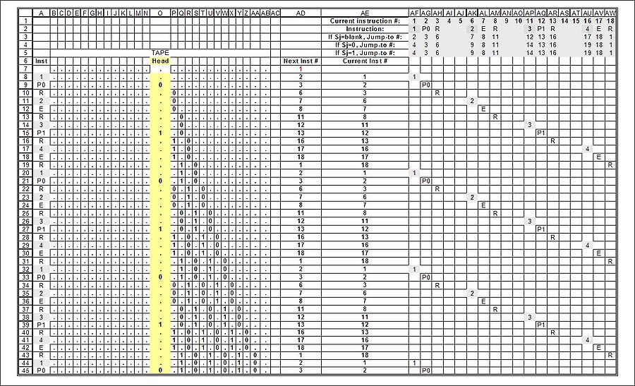
The same "run" with all the intermediate tape-printing and movements is shown here:

A close look at the table reveals certain problems with Turing's own example—not all the symbols are accounted for.

For example, suppose his tape was not initially blank. What would happen?
The Turing machine would read different values than the intended values.

A copy subroutine

This is a very important subroutine used in the "multiply" routine.

The example Turing machine handles a string of 0s and 1s, with 0 represented by the blank symbol. Its task is to double any series of 1s encountered on the tape by writing a 0 between them. For example, when the head reads "111", it will write a 0, then "111". The output will be "1110111".

In order to accomplish its task, this Turing machine will need only 5 states of operation, which are called {s₁, s₂, s₃, s₄, s₅}. Each state does 4 actions:

1. Read the symbol under the head
2. Write the output symbol decided by the state
3. Move the tape to the left or to the right decided by the state
4. Switch to the following state decided by the current state

Initial m-configuration (current instruction)	Tape symbol	Print operation	Tape motion	Final m-configuration (next instruction)
s1	0	N	N	H
s1	1	E	R	s2
s2	0	E	R	s3
s2	1	P1	R	s2
s3	0	P1	L	s4
s3	1	P1	R	s3
s4	0	E	L	s5
s4	1	P1	L	s4
s5	0	P1	R	s1
s5	1	P1	L	s5
H	-	-	-

A "run" of the machine sequences through 16 machine-configurations (aka Turing states):

Sequence	Instruction identifier						Head
1	s1	0	0	0	0	1	1	0	0	0	0	0
2	s2	0	0	0	0	0	1	0	0	0	0	0
3	s2	0	0	0	0	0	0	1	0	0	0	0
4	s3	0	0	0	0	0	0	0	1	0	0	0
5	s4	0	0	0	0	1	0	1	0	0	0	0
6	s5	0	0	0	1	0	1	0	0	0	0	0
7	s5	0	0	1	0	1	0	0	0	0	0	0
8	s1	0	0	0	1	0	1	1	0	0	0	0
9	s2	0	0	0	0	1	0	0	1	0	0	0
10	s3	0	0	0	0	0	1	0	0	1	0	0
11	s3	0	0	0	0	0	0	1	0	0	1	0
12	s4	0	0	0	0	1	1	0	0	1	0	0
13	s4	0	0	0	1	1	0	0	1	0	0	0
14	s5	0	0	1	1	0	0	1	0	0	0	0
15	s1	0	0	0	1	1	0	1	1	0	0	0
16	H	0	0	0	1	1	0	1	1	0	0	0

The behavior of this machine can be described as a loop:
it starts out in s₁, replaces the first 1 with a 0, then uses s₂ to move to the right, skipping over 1s and the first 0 encountered. s₃ then skips over the next sequence of 1s (initially there are none) and replaces the first 0 it finds with a 1. s₄ moves back to the left, skipping over 1s until it finds a 0 and switches to s₅. s₅ then moves to the left, skipping over 1s until it finds the 0 that was originally written by s₁.

It replaces that 0 with a 1, moves one position to the right and enters s₁ again for another round of the loop.

This continues until s₁ finds a 0 (this is the 0 in the middle of the two strings of 1s) at which time the machine halts.

Alternative description

Another description sees the problem as how to keep track of how many "1"s there are. We can't use one state for each possible number (a state for each of 0,1,2,3,4,5,6 etc), because then we'd need infinite states to represent all the natural numbers, and the state machine is finite - we'll have to track this using the tape in some way.

The basic way it works is by copying each "1" to the other side, by moving back and forth - it is intelligent enough to remember which part of the trip it is on. In more detail, it carries each "1" across to the other side, by recognizing the separating "0" in the middle, and recognizing the "0" on the other side to know it's reached the end. It comes back using the same method, detecting the middle "0", and then the "0" on the original side. This "0" on the original side is the key to the puzzle of how it keeps track of the number of 1's.

The trick is that before carrying the "1", it marks that digit as "taken" by replacing it with an "0". When it returns, it fills that "0" back in with a "1", then moves on to the next one, marking it with an "0" and repeating the cycle, carrying that "1" across and so on. With each trip across and back, the marker "0" moves one step closer to the centre. This is how it keeps track of how many "1"'s it has taken across.

Interestingly, when it returns, the marker "0" looks like the end of the collection of "1"s to it - any "1"s that have already been taken across are invisible to it (on the other side of the marker "0") and so it is as if it is working on an (N-1) number of "1"s - similar to a proof by Mathematical induction

Mathematical induction

Mathematical induction is a method of mathematical proof typically used to establish that a given statement is true of all natural numbers...

.

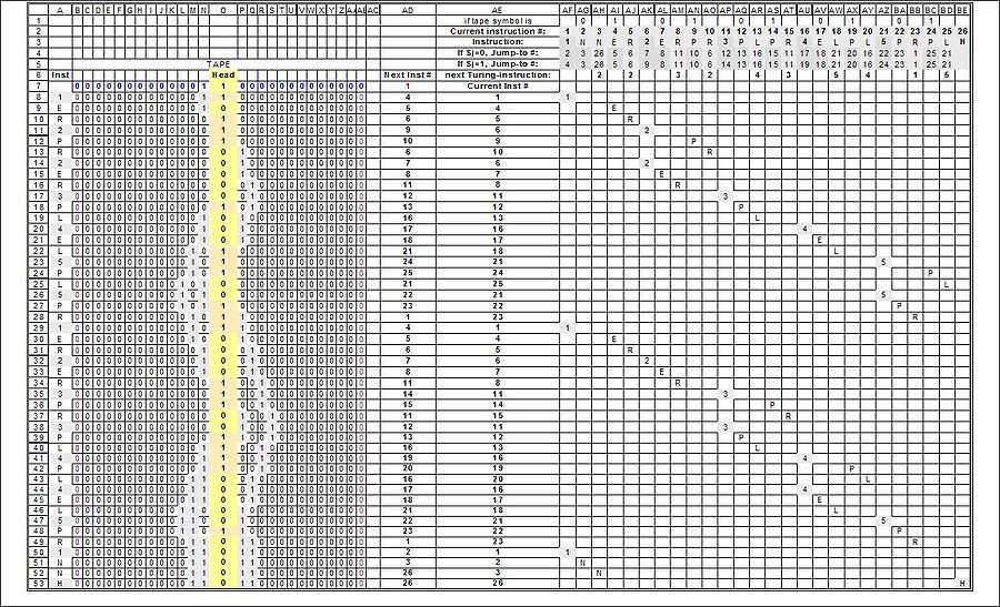
A full "run" showing the results of the intermediate "motions". To see it better click on the image, then click on the higher resolution download:

3-state Busy Beaver

Busy beaver

In computability theory, a busy beaver is a Turing machine that attains the maximum "operational busyness" among all the Turing machines in a certain class...

 

The following Turing table of instructions was derived from Peterson (1988) page 198, Figure 7.15. Peterson moves the head; in the following model the tape moves.

Tape symbol	Current state A			Current state B			Current state C
	Write symbol	Move tape	Next state	Write symbol	Move tape	Next state	Write symbol	Move tape	Next state
0	1	R	B	1	L	A	1	L	B
1	1	L	C	1	R	B	1	N	HALT

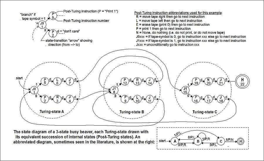
The "state" drawing of the 3-state busy beaver shows the internal sequences of events required to actually perform "the state". As noted above Turing (1937) makes it perfectly clear that this is the proper interpretation of the 5-tuples that describe the instruction (Undecidable, p. 119). For more about the atomization of Turing 5-tuples see Post-Turing machine

Post-Turing machine

A Post–Turing machine is a "program formulation" of an especially simple type of Turing machine, comprising a variant of Emil Post's Turing-equivalent model of computation described below. A Post–Turing machine is a "program formulation" of an especially simple type of Turing machine, comprising a...

:

The following table shows the "compressed" run — just the Turing states:

Sequence	Instruction identifier							Head
1	A	0	0	0	0	0	0	0	0	0	0	0	0	0	0
2	B	0	0	0	0	0	0	0	1	0	0	0	0	0	0
3	A	0	0	0	0	0	1	1	0	0	0	0	0	0	0
4	C	0	0	0	0	1	1	0	0	0	0	0	0	0	0
5	B	0	0	0	1	1	1	0	0	0	0	0	0	0	0
6	A	0	0	1	1	1	1	0	0	0	0	0	0	0	0
7	B	0	0	0	1	1	1	1	1	0	0	0	0	0	0
8	B	0	0	0	0	1	1	1	1	1	0	0	0	0	0
9	B	0	0	0	0	0	1	1	1	1	1	0	0	0	0
10	B	0	0	0	0	0	0	1	1	1	1	1	0	0	0
11	B	0	0	0	0	0	0	0	1	1	1	1	1	0	0
12	A	0	0	0	0	0	1	1	1	1	1	1	0	0	0
13	C	0	0	0	0	1	1	1	1	1	1	0	0	0	0
14	H	0	0	0	0	1	1	1	1	1	1	0	0	0	0

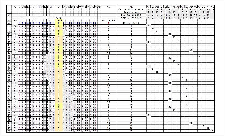
The full "run" of the 3-state busy beaver. The resulting Turing-states (what Turing called the "m-configurations" — "machine-configurations") are shown highlighted in grey in column A, and also under the machine's instructions (columns AF-AU)):