

Reassignment method
Encyclopedia
The method of reassignment is a technique for
sharpening a time-frequency representation
by mapping
the data to time-frequency coordinates that are nearer to
the true region of support
of the
analyzed signal. The method has been independently
introduced by several parties under various names, including
method of reassignment, remapping, time-frequency reassignment,
and modified moving-window method. In
the case of the spectrogram
or the short-time Fourier transform
,
the method of reassignment sharpens blurry
time-frequency data by relocating the data according to
local estimates of instantaneous frequency and group delay.
This mapping to reassigned time-frequency coordinates is
very precise for signals that are separable in time and
frequency with respect to the analysis window.
 Many signals of interest have a distribution of energy that
varies in time and frequency. For example, any sound signal
having a beginning or an end has an energy distribution that
varies in time, and most sounds exhibit considerable
variation in both time and frequency over their duration.
Time-frequency representations are commonly used to analyze
or characterize such signals. They map the one-dimensional
time-domain signal into a two-dimensional function of time
and frequency. A time-frequency representation describes the
variation of spectral energy distribution over time, much as
a musical score describes the variation of musical pitch
over time.
In audio signal analysis, the spectrogram is the most
commonly-used time-frequency representation, probably
because it is well-understood, and immune to so-called
"cross-terms" that sometimes make other time-frequency
representations difficult to interpret. But the windowing
operation required in spectrogram computation introduces an
unsavory tradeoff between time resolution and frequency
resolution, so spectrograms provide a time-frequency
representation that is blurred in time, in frequency, or in
both dimensions. The method of time-frequency reassignment
is a technique for refocussing time-frequency data in a
blurred representation like the spectrogram by mapping the
data to time-frequency coordinates that are nearer to the
true region of support of the analyzed signal.
spectrogram, defined as the squared magnitude of the
short-time Fourier transform. Though the short-time phase
spectrum is known to contain important temporal information
about the signal, this information is difficult to
interpret, so typically, only the short-time magnitude
spectrum is considered in short-time spectral analysis.
As a time-frequency representation, the spectrogram has
relatively poor resolution. Time and frequency resolution
are governed by the choice of analysis window and greater
concentration in one domain is accompanied by greater
smearing in the other.
A time-frequency representation having improved resolution,
relative to the spectrogram, is the Wigner–Ville distribution,
which may be interpreted as a short-time
Fourier transform with a window function that is perfectly
matched to the signal. The Wigner–Ville distribution is
highly-concentrated in time and frequency, but it is also
highly nonlinear and non-local. Consequently, this
distribution is very sensitive to noise, and generates
cross-components that often mask the components of interest,
making it difficult to extract useful information concerning
the distribution of energy in multi-component signals.
Cohen's class
of
bilinear time-frequency representations is a class of
"smoothed" Wigner–Ville distributions, employing a smoothing
kernel that can reduce sensitivity of the distribution to
noise and suppresses cross-components, at the expense of
smearing the distribution in time and frequency. This
smearing causes the distribution to be non-zero in regions
where the true Wigner–Ville distribution shows no energy.
The spectrogram is a member of Cohen's class. It is a
smoothed Wigner–Ville distribution with the smoothing kernel
equal to the Wigner–Ville distribution of the analysis
window. The method of reassignment smoothes the Wigner–Ville
distribution, but then refocuses the distribution back to
the true regions of support of the signal components. The
method has been shown to reduce time and frequency smearing
of any member of Cohen's class
In the case of the reassigned
spectrogram, the short-time phase spectrum is used to
correct the nominal time and frequency coordinates of the
spectral data, and map it back nearer to the true regions of
support of the analyzed signal.
published by Kodera, Gendrin, and de Villedary under the
name of Modified Moving Window Method
Their technique enhances the resolution in time and
frequency of the classical Moving Window Method (equivalent
to the spectrogram) by assigning to each data point a new
time-frequency coordinate that better-reflects the
distribution of energy in the analyzed signal.
In the classical moving window method, a time-domain
signal, is decomposed into a set of
coefficients, , based on a set of elementary signals,
  ,
,
defined

where is a (real-valued) lowpass kernel
function, like the window function in the short-time Fourier
transform. The coefficients in this decomposition are defined
where is the magnitude, and
 the phase, of
 , the Fourier transform of the
signal shifted in time by
and windowed by .
.
 can be reconstructed from the moving window coefficients by
For signals having magnitude spectra,
 , whose time variation is slow
relative to the phase variation, the maximum contribution to
the reconstruction integral comes from the vicinity of the
point satisfying the phase
stationarity condition
or equivalently, around the point defined by
This phenomenon is known in such fields as optics as the
principle of stationary phase,
which states that for periodic or quasi-periodic
signals, the variation of the Fourier phase spectrum not
attributable to periodic oscillation is slow with respect to
time in the vicinity of the frequency of oscillation, and in
surrounding regions the variation is relatively rapid.
Analogously, for impulsive signals, that are concentrated in
time, the variation of the phase spectrum is slow with
respect to frequency near the time of the impulse, and in
surrounding regions the variation is relatively rapid.
In reconstruction, positive and negative contributions to
the synthesized waveform cancel, due to destructive
interference, in frequency regions of rapid phase variation.
Only regions of slow phase variation (stationary phase) will
contribute significantly to the reconstruction, and the
maximum contribution (center of gravity) occurs at the point
where the phase is changing most slowly with respect to time
and frequency.
The time-frequency coordinates thus computed are equal to
the local group delay, ,
,
and local instantaneous frequency, , and are computed from the phase of
the short-time Fourier transform, which is normally ignored
when constructing the spectrogram. These quantities are
local in the sense that they are represent a windowed
and filtered signal that is localized in time and frequency,
and are not global properties of the signal under analysis.
The modified moving window method, or method of
reassignment, changes (reassigns) the point of attribution
of to this point of maximum
contribution , rather than to the point
 at which it is computed. This point is
sometimes called the center of gravity of the
distribution, by way of analogy to a mass distribution. This
analogy is a useful reminder that the attribution of
spectral energy to the center of gravity of its distribution
only makes sense when there is energy to attribute, so the
method of reassignment has no meaning at points where the
spectrogram is zero-valued.
the time and frequency domains. The discrete Fourier
transform is used to compute samples of
of
the Fourier transform from samples of a
of a
time domain signal. The reassignment operations proposed by
Kodera et al. cannot be applied directly to the
discrete short-time Fourier transform data, because partial
derivatives cannot be computed directly on data that is
discrete in time and frequency, and it has been suggested
that this difficulty has been the primary barrier to wider
use of the method of reassignment.
It is possible to approximate the partial derivatives using
finite differences. For example, the phase spectrum can be
evaluated at two nearby times, and the partial derivative
with respect to time be approximated as the difference
between the two values divided by the time difference, as in
For sufficiently small values of and
and
 , and provided that the phase
difference is appropriately "unwrapped", this
finite-difference method yields good approximations to the
partial derivatives of phase, because in regions of the
spectrum in which the evolution of the phase is dominated by
rotation due to sinusoidal oscillation of a single, nearby
component, the phase is a linear function.
Independently of Kodera et al. , Nelson arrived at a similar method for
improving the time-frequency precision of short-time
spectral data from partial derivatives of the short-time phase
spectrum.
It is easily shown that Nelson's
cross spectral surfaces compute an approximation of the derivatives that
is equivalent to the finite differences method.
Auger and Flandrin showed that the method of reassignment, proposed
in the context of the spectrogram by Kodera et al., could be extended to
any member of Cohen's class of time-frequency representations by generalizing the
reassignment operations to
where is the Wigner–Ville
distribution of , and
, and
 is the kernel function that
defines the distribution. They further described an
efficient method for computing the times and frequencies for
the reassigned spectrogram efficiently and accurately
without explicitly computing the partial derivatives of
phase.
In the case of the spectrogram, the reassignment operations
can be computed by
where is the short-time Fourier
transform computed using an analysis window
 ,
, 
is the short-time Fourier transform computed using a
time-weighted anlaysis window and
and
 is the short-time
Fourier transform computed using a time-derivative analysis
window .
.
Using the auxiliary window functions
 and
and
 , the reassignment operations
can be computed at any time-frequency coordinate
 from an algebraic combination of three
Fourier transforms evaluated at . Since
these algorithms operate only on short-time spectral
data evaluated at a single time and frequency, and do not
explicitly compute any derivatives, the reassigned
time-frequency coordinates and
and
 can be computed from
three discrete short-time Fourier transforms evaluated at
 . This gives an efficient
method of computing the reassigned discrete short-time
Fourier transform provided only that the is non-zero. This is not much of a restriction,
since the reassignment operation itself implies that there
is some energy to reassign, and has no meaning when the
distribution is zero-valued.
estimate the amplitudes and phases of the individual
components in a multi-component signal, such as a
quasi-harmonic musical instrument tone. Moreover, the time
and frequency reassignment operations can be used to sharpen
the representation by attributing the spectral energy
reported by the short-time Fourier transform to the point
that is the local center of gravity of the complex energy
distribution.
For a signal consisting of a single component, the
instantaneous frequency can be estimated from the partial
derivatives of phase of any short-time Fourier transform
channel that passes the component. If the signal is to be
decomposed into many components,
and the instantaneous frequency of each component
is defined as the derivative of its phase with respect to time,
that is,

then the instantaneous frequency of each individual component
can be computed from the phase of the response of a filter that passes
that component, provided that no more than
one component lies in the passband of the filter.
This is the property, in the frequency domain, that Nelson
called separability
and is required of all signals so analyzed. If this property is not met, then
the desired multi-component decomposition cannot be achieved,
because the parameters of individual components cannot be
estimated from the short-time Fourier transform. In such
cases, a different analysis window must be chosen so that
the separability criterion is satisfied.
If the components of a signal are separable in frequency
with respect to a particular short-time spectral analysis
window, then the output of each short-time Fourier transform
filter is a filtered version of, at most, a single
dominant (having significant energy) component, and so the
derivative, with respect to time, of the phase of the
 is equal to the derivative with
respect to time, of the phase of the dominant component at
 . Therefore, if a component,
 , having instantaneous frequency
 is the dominant component in the
vicinity of , then the instantaneous
frequency of that component can be computed from the phase
of the short-time Fourier transform evaluated at
 . That is,
Thus, the partial derivative with respect to time of the
phase of the short-time Fourier transform can be used to
compute the instantaneous frequencies of the individual
components in a multi-component signal, provided only that
the components are separable in frequency by the chosen
analysis window.
 Just as each bandpass filter in the short-time Fourier
transform filterbank may pass at most a single complex
exponential component, two temporal events must be
sufficiently separated in time that they do not lie in the
same windowed segment of the input signal. This is the
property of separability in the time domain, and is
equivalent to requiring that the time between two events be
greater than the length of the impulse response of the
short-time Fourier transform filters, the span of non-zero
samples in .
.
Separability in time and in frequency is required of
components to be resolved in a reassigned time-frequency
representation. If the components in a decomposition are
separable in a certain time-frequency
representation, then the components can be resolved by that
time-frequency representation, and using the method of
reassignment, can be characterized with much greater
precision than is possible using classical methods.
In general, there are an infinite number of equally-valid
decompositions for a multi-component signal.
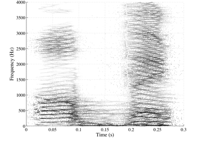
The separability property must be considered in the context of the
desired decomposition. For example, in the analysis of a speech signal,
an analysis window that is long relative to the time between glottal pulses
is sufficient to separate harmonics, but the individual
glottal pulses will be smeared, because
many pulses are covered by each window
(that is, the individual pulses are not separable, in time,
by the chosen analysis window).
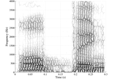
An analysis window that is much shorter than the
time between glottal pulses may resolve the glottal pulses,
because no window spans
more than one pulse, but the harmonic frequencies
are smeared together, because the main lobe of the analysis window
spectrum is wider than the spacing between the harmonics
(that is, the harmonics are not separable, in frequency,
by the chosen analysis window).
sharpening a time-frequency representation
Time-frequency representation
A time–frequency representation is a view of a signal represented over both time and frequency. Time–frequency analysis means analysis into the time–frequency domain provided by a TFR...
by mapping
the data to time-frequency coordinates that are nearer to
the true region of support
Support (mathematics)
In mathematics, the support of a function is the set of points where the function is not zero, or the closure of that set . This concept is used very widely in mathematical analysis...
of the
analyzed signal. The method has been independently
introduced by several parties under various names, including
method of reassignment, remapping, time-frequency reassignment,
and modified moving-window method. In
the case of the spectrogram
Spectrogram
A spectrogram is a time-varying spectral representation that shows how the spectral density of a signal varies with time. Also known as spectral waterfalls, sonograms, voiceprints, or voicegrams, spectrograms are used to identify phonetic sounds, to analyse the cries of animals; they were also...
or the short-time Fourier transform
Short-time Fourier transform
The short-time Fourier transform , or alternatively short-term Fourier transform, is a Fourier-related transform used to determine the sinusoidal frequency and phase content of local sections of a signal as it changes over time....
,
the method of reassignment sharpens blurry
time-frequency data by relocating the data according to
local estimates of instantaneous frequency and group delay.
This mapping to reassigned time-frequency coordinates is
very precise for signals that are separable in time and
frequency with respect to the analysis window.
Introduction
varies in time and frequency. For example, any sound signal
having a beginning or an end has an energy distribution that
varies in time, and most sounds exhibit considerable
variation in both time and frequency over their duration.
Time-frequency representations are commonly used to analyze
or characterize such signals. They map the one-dimensional
time-domain signal into a two-dimensional function of time
and frequency. A time-frequency representation describes the
variation of spectral energy distribution over time, much as
a musical score describes the variation of musical pitch
over time.
In audio signal analysis, the spectrogram is the most
commonly-used time-frequency representation, probably
because it is well-understood, and immune to so-called
"cross-terms" that sometimes make other time-frequency
representations difficult to interpret. But the windowing
operation required in spectrogram computation introduces an
unsavory tradeoff between time resolution and frequency
resolution, so spectrograms provide a time-frequency
representation that is blurred in time, in frequency, or in
both dimensions. The method of time-frequency reassignment
is a technique for refocussing time-frequency data in a
blurred representation like the spectrogram by mapping the
data to time-frequency coordinates that are nearer to the
true region of support of the analyzed signal.
The spectrogram as a time-frequency representation
One of the best-known time-frequency representations is thespectrogram, defined as the squared magnitude of the
short-time Fourier transform. Though the short-time phase
spectrum is known to contain important temporal information
about the signal, this information is difficult to
interpret, so typically, only the short-time magnitude
spectrum is considered in short-time spectral analysis.
As a time-frequency representation, the spectrogram has
relatively poor resolution. Time and frequency resolution
are governed by the choice of analysis window and greater
concentration in one domain is accompanied by greater
smearing in the other.
A time-frequency representation having improved resolution,
relative to the spectrogram, is the Wigner–Ville distribution,
which may be interpreted as a short-time
Fourier transform with a window function that is perfectly
matched to the signal. The Wigner–Ville distribution is
highly-concentrated in time and frequency, but it is also
highly nonlinear and non-local. Consequently, this
distribution is very sensitive to noise, and generates
cross-components that often mask the components of interest,
making it difficult to extract useful information concerning
the distribution of energy in multi-component signals.
Cohen's class
Cohen's class distribution function
Bilinear time–frequency distributions, or quadratic time–frequency distributions, arise in a sub-field field of signal analysis and signal processing called time–frequency signal processing, and, in the statistical analysis of time series data...
of
bilinear time-frequency representations is a class of
"smoothed" Wigner–Ville distributions, employing a smoothing
kernel that can reduce sensitivity of the distribution to
noise and suppresses cross-components, at the expense of
smearing the distribution in time and frequency. This
smearing causes the distribution to be non-zero in regions
where the true Wigner–Ville distribution shows no energy.
The spectrogram is a member of Cohen's class. It is a
smoothed Wigner–Ville distribution with the smoothing kernel
equal to the Wigner–Ville distribution of the analysis
window. The method of reassignment smoothes the Wigner–Ville
distribution, but then refocuses the distribution back to
the true regions of support of the signal components. The
method has been shown to reduce time and frequency smearing
of any member of Cohen's class
In the case of the reassigned
spectrogram, the short-time phase spectrum is used to
correct the nominal time and frequency coordinates of the
spectral data, and map it back nearer to the true regions of
support of the analyzed signal.
The method of reassignment
Pioneering work on the method of reassignment was firstpublished by Kodera, Gendrin, and de Villedary under the
name of Modified Moving Window Method
Their technique enhances the resolution in time and
frequency of the classical Moving Window Method (equivalent
to the spectrogram) by assigning to each data point a new
time-frequency coordinate that better-reflects the
distribution of energy in the analyzed signal.
In the classical moving window method, a time-domain
signal,
is decomposed into a set ofcoefficients,
, based on a set of elementary signals, ,defined
where
is a (real-valued) lowpass kernelfunction, like the window function in the short-time Fourier
transform. The coefficients in this decomposition are defined
where
is the magnitude, and the phase, of, the Fourier transform of thesignal
shifted in time by and windowed by
. can be reconstructed from the moving window coefficients byFor signals having magnitude spectra,
, whose time variation is slowrelative to the phase variation, the maximum contribution to
the reconstruction integral comes from the vicinity of the
point
satisfying the phasestationarity condition
or equivalently, around the point
defined byThis phenomenon is known in such fields as optics as the
principle of stationary phase,
which states that for periodic or quasi-periodic
signals, the variation of the Fourier phase spectrum not
attributable to periodic oscillation is slow with respect to
time in the vicinity of the frequency of oscillation, and in
surrounding regions the variation is relatively rapid.
Analogously, for impulsive signals, that are concentrated in
time, the variation of the phase spectrum is slow with
respect to frequency near the time of the impulse, and in
surrounding regions the variation is relatively rapid.
In reconstruction, positive and negative contributions to
the synthesized waveform cancel, due to destructive
interference, in frequency regions of rapid phase variation.
Only regions of slow phase variation (stationary phase) will
contribute significantly to the reconstruction, and the
maximum contribution (center of gravity) occurs at the point
where the phase is changing most slowly with respect to time
and frequency.
The time-frequency coordinates thus computed are equal to
the local group delay,
,and local instantaneous frequency,
, and are computed from the phase ofthe short-time Fourier transform, which is normally ignored
when constructing the spectrogram. These quantities are
local in the sense that they are represent a windowed
and filtered signal that is localized in time and frequency,
and are not global properties of the signal under analysis.
The modified moving window method, or method of
reassignment, changes (reassigns) the point of attribution
of
to this point of maximumcontribution
, rather than to the point at which it is computed. This point issometimes called the center of gravity of the
distribution, by way of analogy to a mass distribution. This
analogy is a useful reminder that the attribution of
spectral energy to the center of gravity of its distribution
only makes sense when there is energy to attribute, so the
method of reassignment has no meaning at points where the
spectrogram is zero-valued.
Efficient computation of reassigned times and frequencies
In digital signal processing, it is most common to samplethe time and frequency domains. The discrete Fourier
transform is used to compute samples
ofthe Fourier transform from samples
of atime domain signal. The reassignment operations proposed by
Kodera et al. cannot be applied directly to the
discrete short-time Fourier transform data, because partial
derivatives cannot be computed directly on data that is
discrete in time and frequency, and it has been suggested
that this difficulty has been the primary barrier to wider
use of the method of reassignment.
It is possible to approximate the partial derivatives using
finite differences. For example, the phase spectrum can be
evaluated at two nearby times, and the partial derivative
with respect to time be approximated as the difference
between the two values divided by the time difference, as in
For sufficiently small values of
and, and provided that the phasedifference is appropriately "unwrapped", this
finite-difference method yields good approximations to the
partial derivatives of phase, because in regions of the
spectrum in which the evolution of the phase is dominated by
rotation due to sinusoidal oscillation of a single, nearby
component, the phase is a linear function.
Independently of Kodera et al. , Nelson arrived at a similar method for
improving the time-frequency precision of short-time
spectral data from partial derivatives of the short-time phase
spectrum.
It is easily shown that Nelson's
cross spectral surfaces compute an approximation of the derivatives that
is equivalent to the finite differences method.
Auger and Flandrin showed that the method of reassignment, proposed
in the context of the spectrogram by Kodera et al., could be extended to
any member of Cohen's class of time-frequency representations by generalizing the
reassignment operations to
where
is the Wigner–Villedistribution of
, and is the kernel function thatdefines the distribution. They further described an
efficient method for computing the times and frequencies for
the reassigned spectrogram efficiently and accurately
without explicitly computing the partial derivatives of
phase.
In the case of the spectrogram, the reassignment operations
can be computed by
where
is the short-time Fouriertransform computed using an analysis window
, is the short-time Fourier transform computed using a
time-weighted anlaysis window
and is the short-timeFourier transform computed using a time-derivative analysis
window
.Using the auxiliary window functions
and, the reassignment operationscan be computed at any time-frequency coordinate
from an algebraic combination of threeFourier transforms evaluated at
. Sincethese algorithms operate only on short-time spectral
data evaluated at a single time and frequency, and do not
explicitly compute any derivatives, the reassigned
time-frequency coordinates
and can be computed fromthree discrete short-time Fourier transforms evaluated at
. This gives an efficientmethod of computing the reassigned discrete short-time
Fourier transform provided only that the
is non-zero. This is not much of a restriction,since the reassignment operation itself implies that there
is some energy to reassign, and has no meaning when the
distribution is zero-valued.
Separability
The short-time Fourier transform can often be used toestimate the amplitudes and phases of the individual
components in a multi-component signal, such as a
quasi-harmonic musical instrument tone. Moreover, the time
and frequency reassignment operations can be used to sharpen
the representation by attributing the spectral energy
reported by the short-time Fourier transform to the point
that is the local center of gravity of the complex energy
distribution.
For a signal consisting of a single component, the
instantaneous frequency can be estimated from the partial
derivatives of phase of any short-time Fourier transform
channel that passes the component. If the signal is to be
decomposed into many components,
and the instantaneous frequency of each component
is defined as the derivative of its phase with respect to time,
that is,
then the instantaneous frequency of each individual component
can be computed from the phase of the response of a filter that passes
that component, provided that no more than
one component lies in the passband of the filter.
This is the property, in the frequency domain, that Nelson
called separability
and is required of all signals so analyzed. If this property is not met, then
the desired multi-component decomposition cannot be achieved,
because the parameters of individual components cannot be
estimated from the short-time Fourier transform. In such
cases, a different analysis window must be chosen so that
the separability criterion is satisfied.
If the components of a signal are separable in frequency
with respect to a particular short-time spectral analysis
window, then the output of each short-time Fourier transform
filter is a filtered version of, at most, a single
dominant (having significant energy) component, and so the
derivative, with respect to time, of the phase of the
is equal to the derivative withrespect to time, of the phase of the dominant component at
. Therefore, if a component,, having instantaneous frequency is the dominant component in thevicinity of
, then the instantaneousfrequency of that component can be computed from the phase
of the short-time Fourier transform evaluated at
. That is,Thus, the partial derivative with respect to time of the
phase of the short-time Fourier transform can be used to
compute the instantaneous frequencies of the individual
components in a multi-component signal, provided only that
the components are separable in frequency by the chosen
analysis window.
transform filterbank may pass at most a single complex
exponential component, two temporal events must be
sufficiently separated in time that they do not lie in the
same windowed segment of the input signal. This is the
property of separability in the time domain, and is
equivalent to requiring that the time between two events be
greater than the length of the impulse response of the
short-time Fourier transform filters, the span of non-zero
samples in
.Separability in time and in frequency is required of
components to be resolved in a reassigned time-frequency
representation. If the components in a decomposition are
separable in a certain time-frequency
representation, then the components can be resolved by that
time-frequency representation, and using the method of
reassignment, can be characterized with much greater
precision than is possible using classical methods.
In general, there are an infinite number of equally-valid
decompositions for a multi-component signal.
The separability property must be considered in the context of the
desired decomposition. For example, in the analysis of a speech signal,
an analysis window that is long relative to the time between glottal pulses
is sufficient to separate harmonics, but the individual
glottal pulses will be smeared, because
many pulses are covered by each window
(that is, the individual pulses are not separable, in time,
by the chosen analysis window).
An analysis window that is much shorter than the
time between glottal pulses may resolve the glottal pulses,
because no window spans
more than one pulse, but the harmonic frequencies
are smeared together, because the main lobe of the analysis window
spectrum is wider than the spacing between the harmonics
(that is, the harmonics are not separable, in frequency,
by the chosen analysis window).
Further reading
- S. A. Fulop and K. Fitz, A spectrogram for the twenty-first century, Acoustics Today, vol. 2, no. 3, pp. 26–33, 2006.
- S. A. Fulop and K. Fitz, Algorithms for computing the time-corrected instantaneous frequency (reassigned) spectrogram, with applications, Journal of the Acoustical Society of America, vol. 119, pp. 360 – 371, Jan 2006.
External links
- TFTB — Time-Frequency ToolBox
- SPEAR - Sinusoidal Partial Editing Analysis and Resynthesis
- Loris - Open-source software for sound modeling and morphing
- SRA - A web-based research tool for spectral and roughness analysis of sound signals (supported by a Northwest Academic Computing Consortium grant to J. Middleton, Eastern Washington University)