Shape context
Encyclopedia
Shape context is the term given by Serge Belongie and Jitendra Malik
to the feature descriptor they first proposed in their paper "Matching with Shape Contexts" in 2000. Shape context can be used in object recognition
.
is defined to be the shape context of . The bins are normally taken to be uniform in log-polar space. The fact that the shape context is a rich and discriminative descriptor can be seen in the figure below, in which the shape contexts of two different versions of the letter "A" are shown.
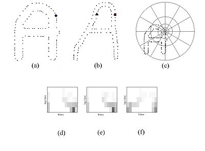
(a) and (b) are the sampled edge points of the two shapes. (c) is the diagram of the log-polar bins used to compute the shape context. (d) is the shape context for the circle, (e) is that for the diamond, and (f) is that for the triangle. As can be seen, since (d) and (e) are the shape contexts for two closely related points, they are quite similar, while the shape context in (f) is very different.
Now in order for a feature descriptor to be useful, it needs to have certain invariances. In particular it needs to be invariant to translation, scale, small perturbations, and depending on application rotation. Translational invariance come naturally to shape context. Scale invariance is obtained by normalizing all radial distances by the mean distance between all the point pairs in the shape although the median distance can also be used. Shape contexts are empirically demonstrated to be robust to deformations, noise, and outliers using synthetic point set matching experiments.
One can provide complete rotation invariance in shape contexts. One way is to measure angles at each point relative to the direction of the tangent at that point (since the points are chosen on edges). This results in a completely rotationally invariant descriptor. But of course this is not always desired since some local features lose their discriminative power if not measured relative to the same frame. Many applications in fact forbid rotation invariance e.g. distinguishing a "6" from a "9".
s. It is preferable to sample the shape with roughly uniform spacing, though it is not critical .
The values of this range from 0 to 1 .
In addition to the shape context cost, an extra cost based on the appearance can be added. For instance, it could be a measure of tangent angle dissimilarity (particularly useful in digit recognition):
Jitendra Malik
Jitendra Malik is a researcher in computer vision, the Arthur J. Chick Professor of Electrical Engineering and Computer Science at the University of California, Berkeley....
to the feature descriptor they first proposed in their paper "Matching with Shape Contexts" in 2000. Shape context can be used in object recognition
Object recognition
Object recognition in computer vision is the task of finding a given object in an image or video sequence. Humans recognize a multitude of objects in images with little effort, despite the fact that the image of the objects may vary somewhat in different view points, in many different sizes / scale...
.
Theory
The shape context is intended to be a way of describing shapes that allows for measuring shape similarity and the recovering of point correspondences . The basic idea is to pick n points on the contours of a shape. For each point pi on the shape, consider the n − 1 vectors obtained by connecting pi to all other points. The set of all these vectors is a rich description of the shape localized at that point but is far too detailed. The key idea is that the distribution over relative positions is a robust, compact, and highly discriminative descriptor. So, for the point pi, the coarse histogram of the relative coordinates of the remaining n − 1 points,
is defined to be the shape context of
. The bins are normally taken to be uniform in log-polar space. The fact that the shape context is a rich and discriminative descriptor can be seen in the figure below, in which the shape contexts of two different versions of the letter "A" are shown.(a) and (b) are the sampled edge points of the two shapes. (c) is the diagram of the log-polar bins used to compute the shape context. (d) is the shape context for the circle, (e) is that for the diamond, and (f) is that for the triangle. As can be seen, since (d) and (e) are the shape contexts for two closely related points, they are quite similar, while the shape context in (f) is very different.
Now in order for a feature descriptor to be useful, it needs to have certain invariances. In particular it needs to be invariant to translation, scale, small perturbations, and depending on application rotation. Translational invariance come naturally to shape context. Scale invariance is obtained by normalizing all radial distances by the mean distance
between all the point pairs in the shape although the median distance can also be used. Shape contexts are empirically demonstrated to be robust to deformations, noise, and outliers using synthetic point set matching experiments.One can provide complete rotation invariance in shape contexts. One way is to measure angles at each point relative to the direction of the tangent at that point (since the points are chosen on edges). This results in a completely rotationally invariant descriptor. But of course this is not always desired since some local features lose their discriminative power if not measured relative to the same frame. Many applications in fact forbid rotation invariance e.g. distinguishing a "6" from a "9".
Use in shape matching
A complete system that uses shape contexts for shape matching consists of the following steps (which will be covered in more detail in the Details of Implementation section):- Randomly select a set of points that lie on the edges of a known shape and another set of points on an unknown shape.
- Compute the shape context of each point found in step 1.
- Match each point from the known shape to a point on an unknown shape. To minimize the cost of matching, first choose a transformation (e.g. affineAffine transformationIn geometry, an affine transformation or affine map or an affinity is a transformation which preserves straight lines. It is the most general class of transformations with this property...
, thin plate splineThin plate splineThis is a brief derivation for the closed form solutions for smoothing Thin Plate Spline. Details about these splines can be found in ....
, etc) that warps the edges of the known shape to the unknown (essentially aligning the two shapes). Then select the point on the unknown shape that most closely corresponds to each warped point on the known shape. - Calculate the "shape distance" between each pair of points on the two shapes. Use a weighted sum of the shape context distance, the image appearance distance, and the bending energy (a measure of how much transformation is required to bring the two shapes into alignment).
- To identify the unknown shape, use a nearest-neighbor classifierNearest neighbor searchNearest neighbor search , also known as proximity search, similarity search or closest point search, is an optimization problem for finding closest points in metric spaces. The problem is: given a set S of points in a metric space M and a query point q ∈ M, find the closest point in S to q...
to compare its shape distance to shape distances of known objects.
Step 1: Finding a list of points on shape edges
The approach essentially assumes that the shape of an object is essentially captured by a finite subset of the points on the internal or external contours on the object. These can be simply obtained using the Canny edge detector and picking a random set of points from the edges. Note that these points need not and in general do not correspond to key-points such as maxima of curvature or inflection pointInflection point
In differential calculus, an inflection point, point of inflection, or inflection is a point on a curve at which the curvature or concavity changes sign. The curve changes from being concave upwards to concave downwards , or vice versa...
s. It is preferable to sample the shape with roughly uniform spacing, though it is not critical .
Step 2: Computing the shape context
This step is described in detail in the Theory section.Step 3: Computing the cost matrix
Consider two points p and q that have normalized K-bin histograms (i.e. shape contexts) g(k) and h(k). As shape contexts are distributions represented as histograms, it is natural to use the χ2 test statistic as the "shape context cost" of matching the two points:
The values of this range from 0 to 1 .
In addition to the shape context cost, an extra cost based on the appearance can be added. For instance, it could be a measure of tangent angle dissimilarity (particularly useful in digit recognition):
-

This is half the length of the chord in unit circle between the unit vectors with angles and
and  . Its values also range from 0 to 1. Now the total cost of matching the two points could be a weighted-sum of the two costs:
Now for each point pi on the first shape and a point qj on the second shape, calculate the cost as described and call it Ci,j. This is the cost matrix.
Step 4: Finding the matching that minimizes total cost
Now, a one-to-one matching pi that matches each point pi on shape 1 and qj on shape 2 that minimizes the total cost of matching,
is needed. This can be done in time using the Hungarian method, although there are more efficient algorithms.
To have robust handling of outliers, one can add "dummy" nodes that have a constant but reasonably large cost of matching to the cost matrix. This would cause the matching algorithm to match outliers to a "dummy" if there is no real match.
Step 5: Modeling transformation
Given the set of correspondences between a finite set of points on the two shapes, a transformation can be estimated to map any point from one shape to the other. There are several choices for this transformation, described below.
Affine
The affine modelAffine transformationIn geometry, an affine transformation or affine map or an affinity is a transformation which preserves straight lines. It is the most general class of transformations with this property...
is a standard choice: . The least squaresLeast squaresThe method of least squares is a standard approach to the approximate solution of overdetermined systems, i.e., sets of equations in which there are more equations than unknowns. "Least squares" means that the overall solution minimizes the sum of the squares of the errors made in solving every...
solution for the matrix and the translational offset vector o is obtained by:
-

Where with a similar expression for
  .
.  is the pseudoinverse of
  .
.
Thin plate spline
The thin plate spline (TPS)Thin plate splineThis is a brief derivation for the closed form solutions for smoothing Thin Plate Spline. Details about these splines can be found in ....
model is the most widely used model for transformations when working with shape contexts. A 2D transformation can be separated into two TPS function to model a coordinate transform:
where each of the ƒx and ƒy have the form:
-

and the kernel function is defined by
  . The exact details of how to solve for the parameters can be found elsewhere but it essentially involves solving a linear system of equations. The bending energy (a measure of how much transformation is needed to align the points) will also be easily obtained.
Regularized TPS
The TPS formulation above has exact matching requirement for the pairs of points on the two shapes. For noisy data, it is best to relax this exact requirement. If we let denote the target function values at corresponding locations
  (Note that for
  ,
,  would
would  the x-coordinate of the point corresponding to
  and for
  it would be the y-coordinate,
  ), relaxing the requirement amounts to minimizing
where is the bending energy and
  is called the regularization parameter. This ƒ that minimizes H[ƒ] can be found in a fairly straightforward way. If one uses normalize coordinates for
  , then scale invariance is kept. However, if one uses the original non-normalized coordinates, then the regularization parameter needs to be normalized.
Note that in many cases, regardless of the transformation used, the initial estimate of the correspondences contains some errors which could reduce the quality of the transformation. If we iterate the steps of finding correspondences and estimating transformations (i.e. repeating steps 2–5 with the newly transformed shape) we can overcome this problem. Typically, three iterations are all that is needed to obtain reasonable results.
Step 6: Computing the shape distance
Now, a shape distance between two shapes and
and  . This distance is going to be a weighted sum of three potential terms:
Shape context distance: this is the symmetric sum of shape context matching costs over best matching points:
where T(·) is the estimated TPS transform that maps the points in Q to those in P.
Appearance cost: After establishing image correspondences and properly warping one image to match the other, one can define an appearance cost as the sum of squared brightness differences in Gaussian windowsGaussian filterIn electronics and signal processing, a Gaussian filter is a filter whose impulse response is a Gaussian function. Gaussian filters are designed to give no overshoot to a step function input while minimizing the rise and fall time. This behavior is closely connected to the fact that the Gaussian...
around corresponding image points:
where and
and  are the gray-level images (
 is the image after warping) and
  is a Gaussian windowing function.
Transformation cost: The final cost measures how much transformation is necessary to bring the two images into alignment. In the case of TPS, it is assigned to be the bending energy.
Now that we have a way of calculating the distance between two shapes, we can use a nearest neighborK-nearest neighbor algorithmIn pattern recognition, the k-nearest neighbor algorithm is a method for classifying objects based on closest training examples in the feature space. k-NN is a type of instance-based learning, or lazy learning where the function is only approximated locally and all computation is deferred until...
classifier (k-NN) with distance defined as the shape distance calculated here. The results of applying this to different situations is given in the following section.
Digit recognition
The authors Serge Belongie and Jitendra MalikJitendra MalikJitendra Malik is a researcher in computer vision, the Arthur J. Chick Professor of Electrical Engineering and Computer Science at the University of California, Berkeley....
tested their approach on the MNIST dataset of handwritten digits. Currently, more than 50 algorithms have been tested on the database. The database has a training set of 60,000 examples, and a test set of 10,000 examples. The error rate for this approach was 0.63% using 20,000 training examples and 3-NN. At the time of publication, this error rate was the lowest. Currently, the lowest error rate is 0.35%.
Silhouette similarity-based retrieval
The authors experimented with the MPEG-7 shape silhouette database, performing Core Experiment CE-Shape-1 part B, which measures performance of similarity-based retrieval. The database has 70 shape categories and 20 images per shape category. Performance of a retrieval scheme is tested by using each image as a query and counting the number of correct images in the top 40 matches. For this experiment, the authors increased the amount of points sampled from each shape. Also, since the shapes in the database sometimes were rotated or flipped, the authors took defined the distance between a reference shape and query shape to be minimum shape distance between the query shape and either the unchanged reference, the vertically flipped, or the reference horizontally flipped . With these changes, they obtained a retrieval rate of 76.45%, which by 2002 was the best.
3D object recognition
The next experiment performed on shape contexts involved the 20 common household objects in the Columbia Object Image Library (COIL-20). Each object has 72 views in the database. In the experiment, the method was trained on a number of equally spaced views for each object and the remaining views were used for testing. A 1-NN classifier was used. The authors also developed an editing algorithm based on shape context similarity and k-medoid clustering that improved on their performance .
Trademark retrieval
Shape contexts were used to retrieve the closest matching trademarks from a database to a query trademark (useful in detecting trademark infringement). No visually similar trademark was missed by the algorithm (verified manually by the authors).
External links
-
-
-