
Radial basis function network
Encyclopedia
A radial basis function network is an artificial neural network
that uses radial basis function
s as activation functions. It is a linear combination
of radial basis functions. They are used in function approximation
, time series prediction, and control
.
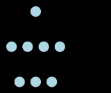
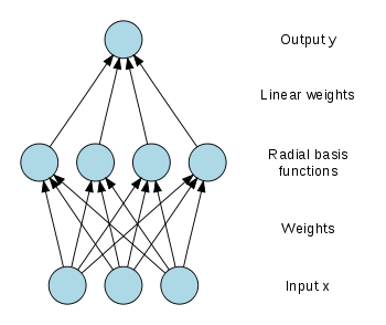 Radial basis function (RBF) networks typically have three layers: an input layer, a hidden layer with a non-linear RBF activation function and a linear output layer. The output,
  , of the network is thus
where N is the number of neurons in the hidden layer, is the center vector for neuron i, and
  are the weights of the linear output neuron. In the basic form all inputs are connected to each hidden neuron. The norm is typically taken to be the Euclidean distance
(though Mahalanobis distance
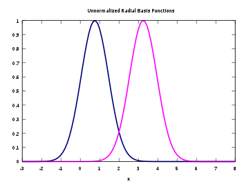
appears to perform better in general) and the basis function is taken to be Gaussian
 .
.
The Gaussian basis functions are local in the sense that
i.e. changing parameters of one neuron has only a small effect for input values that are far away from the center of that neuron.
RBF networks are universal approximators on a compact subset of . This means that a RBF network with enough hidden neurons can approximate any continuous function with arbitrary precision.
The weights ,
,  , and
, and  are determined in a manner that optimizes the fit between
  and the data.
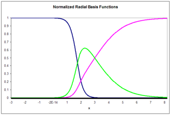
where

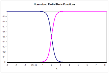
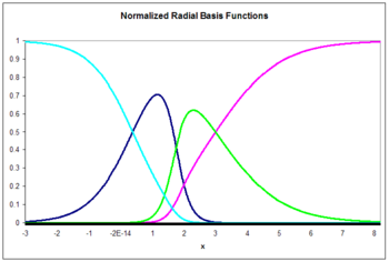
is known as a "normalized radial basis function".
approximation for the joint probability density

where the weights and
and  are exemplars from the data and we require the kernels to be normalized
and .
.
 The probability densities in the input and output spaces are

and
The expectation of y given an input is
is
where
is the conditional probability of y given .
.
The conditional probability is related to the joint probability through Bayes theorem
which yields
 .
.
This becomes
when the integrations are performed.
models. In that case the architectures become, to first order,
and
in the unnormalized and normalized cases, respectively. Here are weights to be determined. Higher order linear terms are also possible.
This result can be written
where
and

in the unnormalized case and
in the normalized case.
Here is a Kronecker delta function defined as
 .
.
 , the output weights
  , and the RBF width parameters
  . In the sequential training of the weights are updated at each time step as data streams in.
For some tasks it makes sense to define an objective function and select the parameter values that minimize its value. The most common objective function is the least squares function
where .
.
We have explicitly included the dependence on the weights. Minimization of the least squares objective function by optimal choice of weights optimizes accuracy of fit.
There are occasions in which multiple objectives, such as smoothness as well as accuracy, must be optimized. In that case it is useful to optimize a regularized objective function such as

where
and
where optimization of S maximizes smoothness and is known as a regularization
parameter.
 when the values of that function are known on finite number of points:
  . Taking the known points
  to be the centers of the radial basis functions and evaluating the values of the basis functions at the same points
  the weights can be solved from the equation
end
It can be shown that the interpolation matrix in the above equation is non-singular, if the points are distinct, and thus the weights
  can be solved by simple linear algebra:
or classification the optimization is somewhat more complex because there is no obvious choice for the centers. The training is typically done in two phases first fixing the width and centers and then the weights. This can be justified by considering the different nature of the non-linear hidden neurons versus the linear output neuron.
the samples and choosing the cluster means as the centers.
The RBF widths are usually all fixed to same value which is proportional to the maximum distance between the chosen centers.
 have been fixed, the weights that minimize the error at the output are computed with a linear pseudoinverse
solution: ,
,
where the entries of G are the values of the radial basis functions evaluated at the points :
:  .
.
The existence of this linear solution means that unlike Multi-Layer Perceptron (MLP) networks the RBF networks have a unique local minimum (when the centers are fixed).
. In gradient descent training, the weights are adjusted at each time step by moving them in a direction opposite from the gradient of the objective function (thus allowing the minimum of the objective function to be found),
where is a "learning parameter."
For the case of training the linear weights, , the algorithm becomes

in the unnormalized case and

in the normalized case.
For local-linear-architectures gradient-descent training is

 and
and  , the algorithm becomes
in the unnormalized case and

in the normalized case and
in the local-linear case.
For one basis function, projection operator training reduces to Newton's method
.
, which maps the unit interval onto itself. It can be used to generate a convenient prototype data stream. The logistic map can be used to explore function approximation
, time series prediction, and control theory
. The map originated from the field of population dynamics
and became the prototype for chaotic
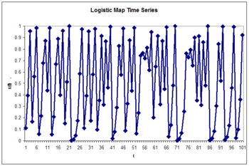
time series. The map, in the fully chaotic regime, is given by
where t is a time index. The value of x at time t+1 is a parabolic function of x at time t. This equation represents the underlying geometry of the chaotic time series generated by the logistic map.
Generation of the time series from this equation is the forward problem. The examples here illustrate the inverse problem
; identification of the underlying dynamics, or fundamental equation, of the logistic map from exemplars of the time series. The goal is to find an estimate

for f.
where
 .
.
Since the input is a scalar
rather than a vector, the input dimension is one. We choose the number of basis functions as N=5 and the size of the training set to be 100 exemplars generated by the chaotic time series. The weight is taken to be a constant equal to 5. The weights
  are five exemplars from the time series. The weights
  are trained with projection operator training:

where the learning rate is taken to be 0.3. The training is performed with one pass through the 100 training points. The rms error
is 0.15.

where
 .
.
Again:
 .
.
Again, we choose the number of basis functions as five and the size of the training set to be 100 exemplars generated by the chaotic time series. The weight is taken to be a constant equal to 6. The weights
  are five exemplars from the time series. The weights
  are trained with projection operator training:
where the learning rate is again taken to be 0.3. The training is performed with one pass through the 100 training points. The rms error
on a test set of 100 exemplars is 0.084, smaller than the unnormalized error. Normalization yields accuracy improvement. Typically accuracy with normalized basis functions increases even more over unnormalized functions as input dimensionality increases.


 .
.
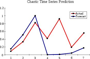
A comparison of the actual and estimated time series is displayed in the figure. The estimated times series starts out at time zero with an exact knowledge of x(0). It then uses the estimate of the dynamics to update the time series estimate for several time steps.
Note that the estimate is accurate for only a few time steps. This is a general characteristic of chaotic time series. This is a property of the sensitive dependence on initial conditions common to chaotic time series. A small initial error is amplified with time. A measure of the divergence of time series with nearly identical initial conditions is known as the Lyapunov exponent
.
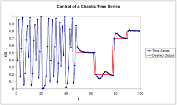 We assume the output of the logistic map can be manipulated through a control parameter
  such that
 .
.
The goal is to choose the control parameter in such a way as to drive the time series to a desired output . This can be done if we choose the control paramer to be
where

is an approximation to the underlying natural dynamics of the system.
The learning algorithm is given by
where
 .
.
Artificial neural network
An artificial neural network , usually called neural network , is a mathematical model or computational model that is inspired by the structure and/or functional aspects of biological neural networks. A neural network consists of an interconnected group of artificial neurons, and it processes...
that uses radial basis function
Radial basis function
A radial basis function is a real-valued function whose value depends only on the distance from the origin, so that \phi = \phi; or alternatively on the distance from some other point c, called a center, so that \phi = \phi...
s as activation functions. It is a linear combination
Linear combination
In mathematics, a linear combination is an expression constructed from a set of terms by multiplying each term by a constant and adding the results...
of radial basis functions. They are used in function approximation
Function approximation
The need for function approximations arises in many branches of applied mathematics, and computer science in particular. In general, a function approximation problem asks us to select a function among a well-defined class that closely matches a target function in a task-specific way.One can...
, time series prediction, and control
Control theory
Control theory is an interdisciplinary branch of engineering and mathematics that deals with the behavior of dynamical systems. The desired output of a system is called the reference...
.
Network architecture
, of the network is thuswhere N is the number of neurons in the hidden layer,
is the center vector for neuron i, and are the weights of the linear output neuron. In the basic form all inputs are connected to each hidden neuron. The norm is typically taken to be the Euclidean distanceEuclidean distance
In mathematics, the Euclidean distance or Euclidean metric is the "ordinary" distance between two points that one would measure with a ruler, and is given by the Pythagorean formula. By using this formula as distance, Euclidean space becomes a metric space...
(though Mahalanobis distance
Mahalanobis distance
In statistics, Mahalanobis distance is a distance measure introduced by P. C. Mahalanobis in 1936. It is based on correlations between variables by which different patterns can be identified and analyzed. It gauges similarity of an unknown sample set to a known one. It differs from Euclidean...
appears to perform better in general) and the basis function is taken to be Gaussian
.The Gaussian basis functions are local in the sense that
i.e. changing parameters of one neuron has only a small effect for input values that are far away from the center of that neuron.
RBF networks are universal approximators on a compact subset of
. This means that a RBF network with enough hidden neurons can approximate any continuous function with arbitrary precision.The weights
, , and are determined in a manner that optimizes the fit between and the data.Normalized architecture
In addition to the above unnormalized architecture, RBF networks can be normalized. In this case the mapping iswhere
is known as a "normalized radial basis function".
Theoretical motivation for normalization
There is theoretical justification for this architecture in the case of stochastic data flow. Assume a stochastic kernelStochastic kernel
In statistics, a stochastic kernel estimate is an estimate of the transition function of a stochastic process. Often, this is an estimate of the conditional density function obtained using kernel density estimation...
approximation for the joint probability density
where the weights
and are exemplars from the data and we require the kernels to be normalizedand
.and
The expectation of y given an input
iswhere
is the conditional probability of y given
.The conditional probability is related to the joint probability through Bayes theorem
which yields
.This becomes
when the integrations are performed.
Local linear models
It is sometimes convenient to expand the architecture to include local linearLocal linearity
Local linearity is a property of functions that says — roughly — that the more you zoom in on a point on the graph of the function , the more the graph will look like a straight line. More precisely, a function is locally linear at a point if and only if a tangent line exists at that point...
models. In that case the architectures become, to first order,
and
in the unnormalized and normalized cases, respectively. Here
are weights to be determined. Higher order linear terms are also possible.This result can be written
where
and
in the unnormalized case and
in the normalized case.
Here
is a Kronecker delta function defined as.Training
In a RBF network there are three types of parameters that need to be chosen to adapt the network for a particular task: the center vectors, the output weights , and the RBF width parameters . In the sequential training of the weights are updated at each time step as data streams in.For some tasks it makes sense to define an objective function and select the parameter values that minimize its value. The most common objective function is the least squares function
where
.We have explicitly included the dependence on the weights. Minimization of the least squares objective function by optimal choice of weights optimizes accuracy of fit.
There are occasions in which multiple objectives, such as smoothness as well as accuracy, must be optimized. In that case it is useful to optimize a regularized objective function such as
where
and
where optimization of S maximizes smoothness and
is known as a regularizationRegularization (machine learning)
In statistics and machine learning, regularization is any method of preventing overfitting of data by a model. It is used for solving ill-conditioned parameter-estimation problems...
parameter.
Interpolation
RBF networks can be used to interpolate a function when the values of that function are known on finite number of points: . Taking the known points to be the centers of the radial basis functions and evaluating the values of the basis functions at the same points the weights can be solved from the equationend
It can be shown that the interpolation matrix in the above equation is non-singular, if the points
are distinct, and thus the weights can be solved by simple linear algebra:Function approximation
If the purpose is not to perform strict interpolation but instead more general function approximationFunction approximation
The need for function approximations arises in many branches of applied mathematics, and computer science in particular. In general, a function approximation problem asks us to select a function among a well-defined class that closely matches a target function in a task-specific way.One can...
or classification the optimization is somewhat more complex because there is no obvious choice for the centers. The training is typically done in two phases first fixing the width and centers and then the weights. This can be justified by considering the different nature of the non-linear hidden neurons versus the linear output neuron.
Training the basis function centers
Basis function centers can be randomly sampled among the input instances or obtained by Orthogonal Least Square Learning Algorithm or found by clusteringData clustering
Cluster analysis or clustering is the task of assigning a set of objects into groups so that the objects in the same cluster are more similar to each other than to those in other clusters....
the samples and choosing the cluster means as the centers.
The RBF widths are usually all fixed to same value which is proportional to the maximum distance between the chosen centers.
Pseudoinverse solution for the linear weights
After the centers have been fixed, the weights that minimize the error at the output are computed with a linear pseudoinversePseudoinverse
In mathematics, and in particular linear algebra, a pseudoinverse of a matrix is a generalization of the inverse matrix. The most widely known type of matrix pseudoinverse is the Moore–Penrose pseudoinverse, which was independently described by E. H. Moore in 1920, Arne Bjerhammar in 1951 and...
solution:
,where the entries of G are the values of the radial basis functions evaluated at the points
: .The existence of this linear solution means that unlike Multi-Layer Perceptron (MLP) networks the RBF networks have a unique local minimum (when the centers are fixed).
Gradient descent training of the linear weights
Another possible training algorithm is gradient descentGradient descent
Gradient descent is a first-order optimization algorithm. To find a local minimum of a function using gradient descent, one takes steps proportional to the negative of the gradient of the function at the current point...
. In gradient descent training, the weights are adjusted at each time step by moving them in a direction opposite from the gradient of the objective function (thus allowing the minimum of the objective function to be found),
where
is a "learning parameter."For the case of training the linear weights,
, the algorithm becomesin the unnormalized case and
in the normalized case.
For local-linear-architectures gradient-descent training is
Projection operator training of the linear weights
For the case of training the linear weights, and , the algorithm becomesin the unnormalized case and
in the normalized case and
in the local-linear case.
For one basis function, projection operator training reduces to Newton's method
Newton's method
In numerical analysis, Newton's method , named after Isaac Newton and Joseph Raphson, is a method for finding successively better approximations to the roots of a real-valued function. The algorithm is first in the class of Householder's methods, succeeded by Halley's method...
.
Logistic map
The basic properties of radial basis functions can be illustrated with a simple mathematical map, the logistic mapLogistic map
The logistic map is a polynomial mapping of degree 2, often cited as an archetypal example of how complex, chaotic behaviour can arise from very simple non-linear dynamical equations...
, which maps the unit interval onto itself. It can be used to generate a convenient prototype data stream. The logistic map can be used to explore function approximation
Function approximation
The need for function approximations arises in many branches of applied mathematics, and computer science in particular. In general, a function approximation problem asks us to select a function among a well-defined class that closely matches a target function in a task-specific way.One can...
, time series prediction, and control theory
Control theory
Control theory is an interdisciplinary branch of engineering and mathematics that deals with the behavior of dynamical systems. The desired output of a system is called the reference...
. The map originated from the field of population dynamics
Population dynamics
Population dynamics is the branch of life sciences that studies short-term and long-term changes in the size and age composition of populations, and the biological and environmental processes influencing those changes...
and became the prototype for chaotic
Chaos theory
Chaos theory is a field of study in mathematics, with applications in several disciplines including physics, economics, biology, and philosophy. Chaos theory studies the behavior of dynamical systems that are highly sensitive to initial conditions, an effect which is popularly referred to as the...
time series. The map, in the fully chaotic regime, is given by
where t is a time index. The value of x at time t+1 is a parabolic function of x at time t. This equation represents the underlying geometry of the chaotic time series generated by the logistic map.
Generation of the time series from this equation is the forward problem. The examples here illustrate the inverse problem
Inverse problem
An inverse problem is a general framework that is used to convert observed measurements into information about a physical object or system that we are interested in...
; identification of the underlying dynamics, or fundamental equation, of the logistic map from exemplars of the time series. The goal is to find an estimate
for f.
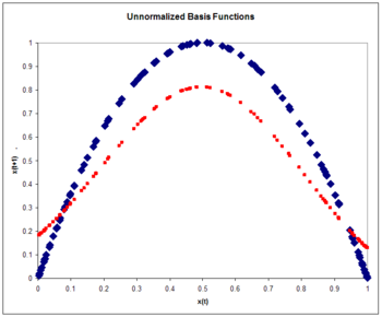
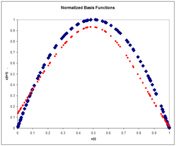
Unnormalized radial basis functions
The architecture iswhere
.Since the input is a scalar
Scalar (mathematics)
In linear algebra, real numbers are called scalars and relate to vectors in a vector space through the operation of scalar multiplication, in which a vector can be multiplied by a number to produce another vector....
rather than a vector, the input dimension is one. We choose the number of basis functions as N=5 and the size of the training set to be 100 exemplars generated by the chaotic time series. The weight
is taken to be a constant equal to 5. The weights are five exemplars from the time series. The weights are trained with projection operator training:where the learning rate
is taken to be 0.3. The training is performed with one pass through the 100 training points. The rms errorMean squared error
In statistics, the mean squared error of an estimator is one of many ways to quantify the difference between values implied by a kernel density estimator and the true values of the quantity being estimated. MSE is a risk function, corresponding to the expected value of the squared error loss or...
is 0.15.
Normalized radial basis functions
The normalized RBF architecture iswhere
.Again:
.Again, we choose the number of basis functions as five and the size of the training set to be 100 exemplars generated by the chaotic time series. The weight
is taken to be a constant equal to 6. The weights are five exemplars from the time series. The weights are trained with projection operator training:where the learning rate
is again taken to be 0.3. The training is performed with one pass through the 100 training points. The rms errorMean squared error
In statistics, the mean squared error of an estimator is one of many ways to quantify the difference between values implied by a kernel density estimator and the true values of the quantity being estimated. MSE is a risk function, corresponding to the expected value of the squared error loss or...
on a test set of 100 exemplars is 0.084, smaller than the unnormalized error. Normalization yields accuracy improvement. Typically accuracy with normalized basis functions increases even more over unnormalized functions as input dimensionality increases.
Time series prediction
Once the underlying geometry of the time series is estimated as in the previous examples, a prediction for the time series can be made by iteration:.A comparison of the actual and estimated time series is displayed in the figure. The estimated times series starts out at time zero with an exact knowledge of x(0). It then uses the estimate of the dynamics to update the time series estimate for several time steps.
Note that the estimate is accurate for only a few time steps. This is a general characteristic of chaotic time series. This is a property of the sensitive dependence on initial conditions common to chaotic time series. A small initial error is amplified with time. A measure of the divergence of time series with nearly identical initial conditions is known as the Lyapunov exponent
Lyapunov exponent
In mathematics the Lyapunov exponent or Lyapunov characteristic exponent of a dynamical system is a quantity that characterizes the rate of separation of infinitesimally close trajectories...
.
Control of a chaotic time series
such that.The goal is to choose the control parameter in such a way as to drive the time series to a desired output
. This can be done if we choose the control paramer to bewhere
is an approximation to the underlying natural dynamics of the system.
The learning algorithm is given by
where
.